
Ecommerce Book Sales Forecast Using Prophet
2025-12-23
This is a time series forecasting pipeline built using Prophet to predict qty and revenue per category using daily ecommerce book sales data from 2020-2022. The model was tuned using a grid search with a time-based holdout split (train before 2022-01-01, test from 2022-01-01 onward) over key Prophet hyperparameters (seasonality mode, changepoint/seasonality priors, yearly seasonality), and enhanced with holiday effects and additional custom seasonalities (monthly/semester). Accuracy was measured using WAPE and MAE at both daily and weekly-aggregated levels, with a 7-day seasonal naive baseline (t-7) used for context.
Objective
Build a forecasting model to predict daily sales quantity (qty) and sales amount (revenue) by product category using historical data from 2020-2022, and evaluate accuracy using WAPE (plus MAE as a secondary metric). The final output includes forecasts for the next 3 years and a summary of model performance and improvement opportunities.
Scopes and Assumptions
This work focuses on the categories Medical and Science & Technology and targets qty and revenue. Holidays/special periods are incorporated as potential demand drivers.
How to Run the Notebook
To run the notebook, follow these instructions:
-
Prerequisites
- Python 3.10+
pipavailable- CPU machine is enough (no GPU required)
-
Create a virtual environment:
python -m venv venv -
Activate the virtual environment:
- Windows:
.\venv\Scripts\activate - Unix/MacOS:
source venv/bin/activate
If you’re running conda
- Windows:
conda create -n myenv python=3.11 -y
- Activate the virtual environment and upgrade
pip
.\.venv\Scripts\Activate.ps1
python -m pip install --upgrade pip
On conda:
conda activate myenv
python -m pip install --upgrade pip
- Install dependencies
python -m pip install -r requirements.txt
Note: Even if ipykernel is listed in requirements.txt, kernel discovery can break due to outdated kernelspec. Refresh it and re-register the kernel:
python -m pip install -U --force-reinstall ipykernel
- Launch Jupyter and open the notebook
Once Jupyter notebook is installed (already in requirements.txt), this works immediately:
jupyter notebook
Then open notebook.ipynb from the browser UI.
- Run the notebook Run cells from top to bottom. If the notebook writes output files (CSVs/models), they will appear in the working directory unless otherwise specified in the notebook.
CPU and Multithreading Notes
This notebook uses multithreading and is intended to run on CPU. It was tested on an AMD Ryzen 5 7600X (6 core / 12 threads) machine.
Methodology
1. Data Ingestion and Validation
Data was ingested from two Excel sources:
- a time-series dataset of e-commerce book sales from 2020-2022. It includes:
- Order Date
- Subject Category
- Sales Amount
- Sales Quantity
- a US holidays calendar
After loading, the date columns were converted to datetime to ensure consistent indexing for later time-series steps. Column names were then standardized to a simple schema (date, category, revenue, qty) to make downstream processing and modeling easier.
Basic validation checks were also performed to confirm the dataset shape and data types, verify the overall date range (2020-01-01 to 2022-12-31), list the available categories, and check that no negative values were present in revenue or qty. The data was then aggregated to daily totals by category and inspected for skipped dates. No skipped dates were found, which confirms a complete daily time series for the selected categories.
2. Data Cleaning and Preprocessing
During preprocessing, the sales data was converted into a modeling-ready time series by aggregating revenue and qty at the day x category level. Dates were normalized to remove time components so that merges and date-based lookups remained consistent.
A US holiday calendar was then used to create calendar-based variables:
is_holiday: flags whether a date is a holidayis_holiday_tmr: flags a day after holiday (to check and model demand spillover after holiday)is_holiday_ytd: flags a day before holiday (to check and model demand spillover before holiday)
No additional cleaning (such as missing date imputation or negative value correction) was needed because the dataset contained a complete daily date range and passed basic sanity checks. Outliers were not removed during preprocessing. Instead, outlier handling was treated as a modeling choice and evaluated later using winsorization (value capping) applied only to the training set. This approach reduces sensitivity to extreme values while avoiding data leakage from the test period.
3. EDA
3.1 Year-to-year Totals
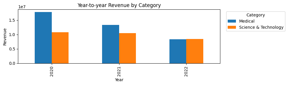
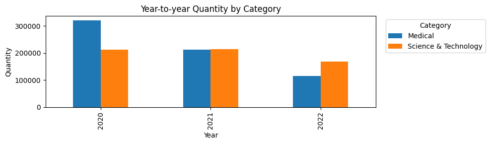
Total revenue and qty by year were compared for each category. This provides a simple sanity check on whether demand levels are stable or shifting over time. Because the dataset covers only about three years, these totals should not be treated as evidence of long-term annual seasonality. However, they help confirm that category-level demand changes across years, which can affect how the model learns trend and seasonality.
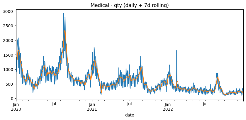
3.2 Daily Series Plot (7d rolling)
Exploratory Data Analysis (EDA) was performed to understand the structure of the sales time series before modeling. For each category and target (revenue , qty), the raw daily series was plotted along with a 7-day rolling mean to reduce day-to-day noise and make the broader pattern easier to see. The example below shows chart for Medical qty.
3.3 Seasonal Decomposition
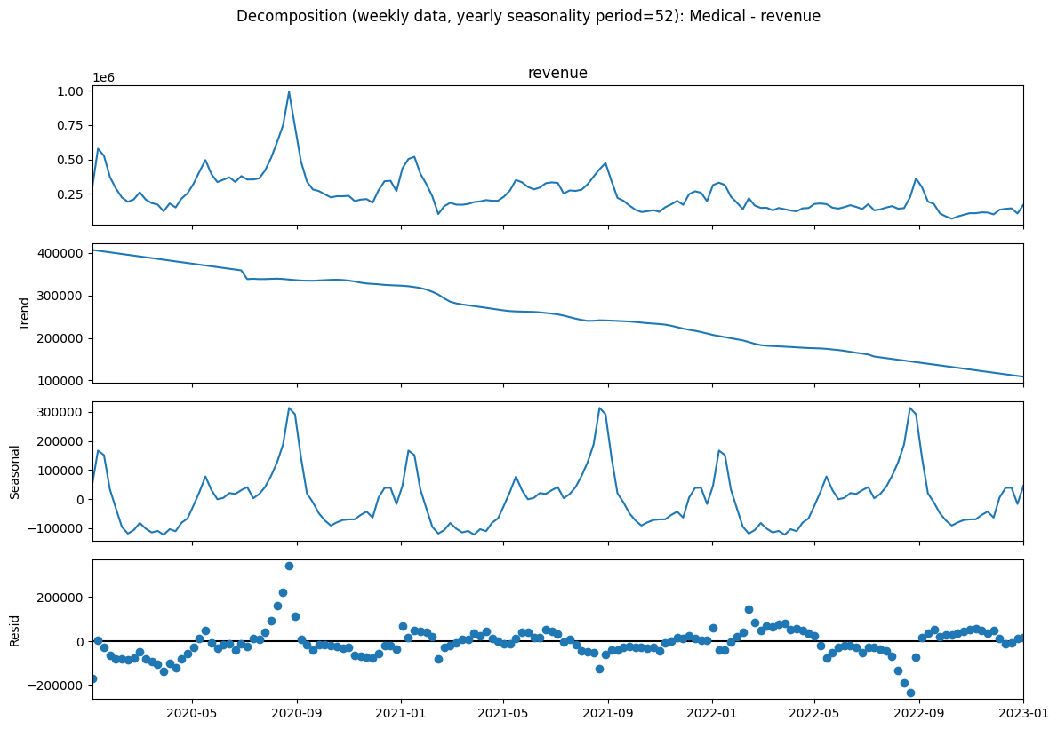
To better understand long-term patterns, a seasonal decomposition was applied to weekly-aggregated data. Daily values were resampled into weekly totals (W-SUN) to reduce day-to-day noise, and the weekly series was decomposed using an additive model with a 52-week period as an approximation of yearly seasonality. The decomposition separates the signal into trend, seasonal, and residual components, making it easier to assess whether an annual cycle is present and how much variation is driven by seasonality versus irregular shocks.
These plots were used as a diagnostic to decide whether adding a yearly component was likely to be helpful. For example, the Medical category showed a clear long-term downward trend, which makes yearly seasonality a reasonable feature to consider during modeling.
3.4 Monthly Pattern Exploration
Month-level seasonality was examined by plotting average demand by month for each category and target using bar charts (see graph below for an example using Science & Technology). This provided a high-level view of whether certain months consistently show higher activity beyond normal fluctuations.
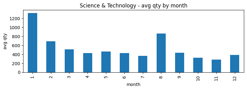
Clear peaks were observed in January and August across both categories and targets, which suggests the presence of recurring seasonal drivers. Given the product categories (Medical and Science & Technology) and the timing of these peaks, a working hypothesis was formed that the spikes may be related to academic semester start periods, when textbooks and related materials are commonly purchased. Because academic calendars can vary, this hypothesis was treated as a tentative explanation and was tested against the data rather than immediately assumed to be true.
To assess whether January and August differ meaningfully from other months (i.e., beyond random variation), a regression-based lift test was performed using log1p(target) as the response and indicator variables for January and August. The log1p transform was used to compress large values and stabilize variance, since the same absolute change can represent very different proportional changes at different baselines. For example, a +50 increase doubles the value from 50 to 100 (100%), but represents only a 1% increase from 5,000 to 5,050.
The lift model also included controls for day-of-week, year, and holiday effects to reduce the risk of attributing routine weekly or calendar-related variation to month effects. The estimated lifts for January and August were positive and statistically significant (see table below), indicating that these months tend to exhibit higher demand even after controlling for standard calendar structure.
| category | target | jan_lift_% | p_jan | aug_lift_% | p_aug | n_obs |
|---|---|---|---|---|---|---|
| Medical | qty |
113.40% | 9e-30 | 87.60% | 1.23e-09 | 1,096 |
| Medical | revenue |
82.70% | 3.63e-17 | 99.20% | 3.05e-12 | 1,096 |
| Science & Technology | qty |
222.00% | 5.21e-42 | 92.10% | 1.08e-06 | 1,096 |
| Science & Technology | revenue |
237.20% | 4.19e-55 | 105.70% | 1.41e-07 | 1,096 |
After January and August were identified as peak months, additional analysis was conducted to determine which week-in-month and day-of-week most consistently correspond to the highest average demand within these months. This step was motivated by the semester start hypothesis: if the peaks are driven by semester timing, the increase would be expected to concentrate in a specific early-month window rather than being evenly distributed across the month. The resulting peak timing patterns were broadly consistent with early semester purchasing behavior. These validated calendar patterns were later used to design additional features so that the forecasting model could better capture recurring demand surges.
| category | month | target | top_week | top_week_mean | top_dow | top_dow_mean |
|---|---|---|---|---|---|---|
| Science & Technology | 1 | revenue |
2 | 81,332.35 | 1 | 93,694.06 |
| Science & Technology | 1 | qty |
2 | 1,554.95 | 1 | 1,812.75 |
| Science & Technology | 8 | revenue |
4 | 70,921.70 | 0 | 56,851.94 |
| Science & Technology | 8 | qty |
4 | 1,330.57 | 0 | 1,066.73 |
| Medical | 1 | revenue |
2 | 69,256.32 | 1 | 68,825.56 |
| Medical | 1 | qty |
2 | 1,244.43 | 1 | 1,285.67 |
| Medical | 8 | revenue |
4 | 78,348.90 | 0 | 82,115.53 |
| Medical | 8 | qty |
4 | 1,226.81 | 0 | 1,281.00 |
3.5 Weekly Pattern Exploration
Weekly seasonality was assessed using autocorrelation. For each category and target, correlations were at lag 1 (short-term dependence) and lag 7 (weekly repeat pattern), and generated Autocorrelation Function (ACF) plots over a wider range of lags. ACF was computed on both log1p(y) and diff(log1p(y)) to separate repeating seasonal structure from trend effects. This analysis was only done on qty because it is less affected by price and product mix than revenue, but the same checks were also used as a loose reference for revenue. Below is an example of ACF plots for Science & Technology.
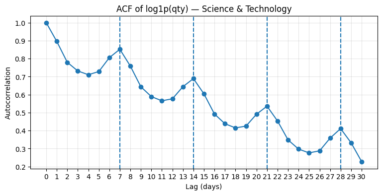
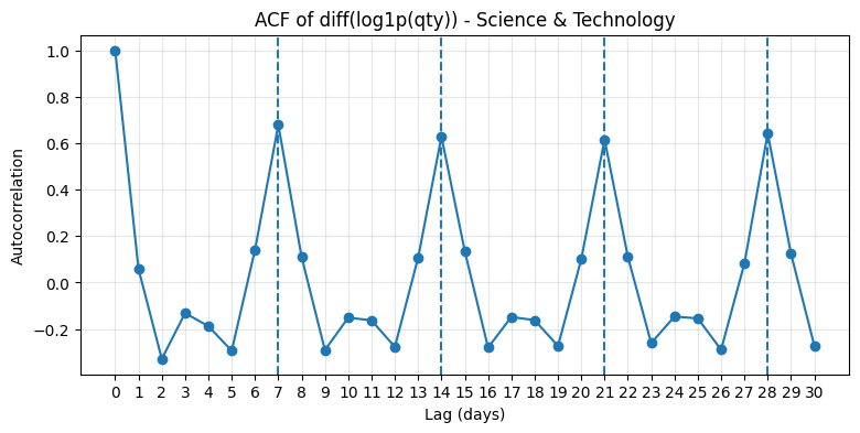
All ACF plots showed clear peaks at lags 7, 14, 21, and 28, which is consistent with a repeating weekly pattern. This supported two modeling choices: enabling weekly seasonality in Prophet and using a 7-day seasonal naive baseline (t-7) as a meaningful reference during evaluation.
3.6 Holiday Effect Analysis
Holiday effects were examined to determine whether sales behavior differs on holiday dates and whether any pre-holiday or post-holiday spillover is present. First, average qty and revenue were compared between holiday and non-holiday dates for each category. This initial check indicated that both quantity and revenue tend to be lower on holidays (see table below), which is consistent with reduced purchasing activity on days when universities and related operations may be closed.
| category | is_holiday | qty | revenue |
|---|---|---|---|
| Science & Technology | 0 (non-holiday) | 544.40 | 27,218.04 |
| Science & Technology | 1 (holiday) | 480.66 | 24,184.46 |
| Medical | 0 (non-holiday) | 594.34 | 36,272.58 |
| Medical | 1 (holiday) | 469.12 | 28,022.22 |
To isolate holiday impacts from normal calendar patterns, a regression-based check was also conducted. The target variable (qty or revenue) was modeled as a function of a holiday indicator and adjacent-day indicators (day before / day after), while controlling for day-of-week and month effects, as well as a simple time trend. Day-of-week controls were included because baseline sales differ systematically across weekdays and many holidays occur on specific weekdays, and without this adjustment, weekday effects could be incorrectly attributed to holidays. Overall, the main holiday indicator remained significant, whereas adjacent day indicators were generally not significant, which suggests limited spillover effects in this dataset. For comprehensive results on this, see table below.
| category | target | coef_holiday | p_holiday | coef_ytd | p_ytd | coef_tmr | p_tmr | n_obs | sig_holiday | sig_ytd | sig_tmr |
|---|---|---|---|---|---|---|---|---|---|---|---|
| Medical | qty |
-185.54 | 4.74e-08 | -12.91 | 0.627964 | -62.28 | 0.038620 | 1,096 | Yes | No | Yes |
| Medical | revenue |
-11,398.87 | 9.78e-09 | -1,262.20 | 0.448626 | -2,938.83 | 0.152958 | 1,096 | Yes | No | No |
| Science & Technology | qty |
-163.91 | 2.53e-04 | 15.11 | 0.773841 | -48.90 | 0.088398 | 1,096 | Yes | No | No |
| Science & Technology | revenue |
-8,203.72 | 2.04e-04 | 810.98 | 0.758792 | -2,354.93 | 0.095431 | 1,096 | Yes | No | No |
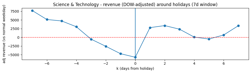
Finally, a day-of-week adjusted holiday profile (7 days before and 7 days after each holiday) was visualized to examine the shape of demand changes surrounding holiday dates after removing typical weekday patterns (see graph below for an example on Science & Technology revenue). The profile supported the conclusion that the primary impact occurs on the holiday itself, with weaker and less consistent patterns on neighboring days. A limitation of this analysis is that all holidays were treated uniformly. Differences between major holidays and minor holidays were not explicitly modeled, and academic breaks were not incorporated into the model at all.
3.7 Model Selection
Prophet was chosen as the main forecasting model because the data is daily time-series data and shows clear calendar-related patterns (weekly cycles, holidays, and repeated peaks). The project also involves several series (category x target), so the model needs to be accurate and reasonably easy to tune and maintain.
Compared with ARIMA/SARIMA/SARIMAX, Prophet was preferred because it can combine trend, seasonality, and holiday/event effects in a more direct way. ARIMA/SARIMA/SARIMAX often needs careful manual setup (for example choosing differencing and AR/MA orders) and this work can become slow when it must be repeated for many series. Although SARIMAX can include both seasonality and exogenous variables, it usually requires more effort to make sure the assumptions fit the data and the parameters are chosen well.
Compared with RNN/LSTM models, Prophet was preferred because only a few years of daily history (2020-2022) are available. Deep learning models usually perform better with larger datasets and can overfit when the data is limited. They also tend to require more complex tuning and are harder to explain, especially when the main drivers are calendar effects.
Compared with XGBoost/LightGBM, Prophet was preferred because tree-based models typically require the time series to be converted into a supervised learning dataset using lag features, rolling features, and many calendar variables. This can work well, but it poses logistical challenge because it increases pipeline complexity and makes it harder to avoid data leakage during evaluation. Prophet already supports forecasting with built-in seasonalities and holiday/event inputs, which makes the overall workflow simpler for this assignment.
Overall, Prophet was selected because it offers a good balance of flexibility, clear handling of calendar effects, and practical implementation across multiple time series.
3.7 Model Design and Training + Testing Procedure
3.7.1 Data Preparation
For each category and target (qty, revenue), the data was reshaped into Prophet’s required format, with ds as the date column and y as the target column. Dates were normalized and a continuous daily index was created. Although no missing dates were observed, the pipeline includes a safeguard that fills any missing dates with zero sales, treating missing records as zero activity rather than missing data.
The data was kept as a daily series rather than aggregated to weekly totals. With only three years of history, weekly aggregation would substantially reduce the number of training observations (1,096 daily points versus ~156 weekly points for each category x target), which can limit the model’s ability to learn trend changes and short-lived calendar effects. Daily modeling also preserves within-week structure and allows event windows (e.g., holidays or semester start periods spanning several days) to be represented more directly. Weekly aggregation was still used during evaluation as a complementary view of accuracy.
Because the target values are non-negative and include large spikes, the target was transformed using log1p(y) during training. As noted earlier, this reduces the influence of extreme values and helps stabilize variance over time. After forecasting, predictions were converted back to the original scale using expm1.
3.7.2 Holiday and Semester-related Events
A holiday calendar was formatted into Prophet’s holiday input structure. In addition to official holidays, custom “semester” events were created to reflect the observed peaks in January and August. For each year, the most typical peak timing within those months was identified using the peak week-in-month and day-of-week. These semester start dates were then added as holiday-like events, with an adjustable forward impact window (7, 14, 21, or 28 days). This allowed the model to represent a demand carryover that persists beyond a single date.
3.7.3 Baseline for Comparison
A simple weekly seasonal naive baseline was used for context. For each day t, the baseline prediction was set to the observed value from t-7 (the same weekday in the previous week). This baseline is appropriate when weekly seasonality is present and provides a clear reference for judging whether Prophet improves performance.
3.7.4 Hyperparameter Tuning (Grid Search with Time-based Holdout)
Hyperparameters were tuned using a grid search. A time-based split was used to preserve the forecasting setting: training data was taken from dates before 2022-01-01, and testing was performed on dates from 2022-01-01 onward. Each parameter combination was fitted on the training period and evaluated on the test period.
The Prophet hyperparameter grid included:
seasonality_mode(additive vs multiplicative)changepoint_prior_scale(trend flexibility)seasonality_prior_scale(strength of seasonality regularization)yearly_seasonality(enabled/disabled)
Additional options were also evaluated during grid search:
- training-only winsorization (
None, 0.99, 0.995, 0.999 quantile caps), to reduce sensitivity to extreme spikes without using test-period information - optional custom seasonalities (monthly and semester-length)
- semester event window length (7/14/21/28 days)
3.7.5 Model Evaluation
Model performance was measured using WAPE and MAE. WAPE was used to provide a scale-normalized accuracy measure that remains stable with low or zero daily values, while MAE was used to report average absolute error in the original units (book units or dollars), which is easier to interpret operationally.
Both metrics were computed at the daily level and also after aggregating values into weekly totals (W-SUN). Weekly evaluation was included because it reduces day-level noise and provides a more stable view of forecast quality.
3.7.6 Final Fit and Forecasting
After tuning, the best-performing configuration (based on WAPE) was selected for each category x target pair. The model was then refit on the full history and used to generate future daily forecasts, including prediction intervals. In the final refit, a log(1+y) transformation was applied to all series. For series whose best configuration used additive seasonality (Science & Technology), Prophet’s logistic growth is additionally used with floor/cap constraints to bound long-horizon forecasts and reduce unrealistic trend decay. For series where the best configuration was multiplicative (Medical), linear growth is retained to preserve the scale-dependent seasonal structure. Forecasts were then converted back to the original scale for reporting. Final models were saved as joblib files for practical usage.
Results
1. Training Results
The table below compares Prophet’s weekly WAPE with a naive baseline (t-7).
| category | target | prophet_WAPE_weekly | baseline7_WAPE_weekly |
|---|---|---|---|
| Medical | qty |
19.90% | 18.22% |
| Medical | revenue |
18.74% | 17.13% |
| Science & Technology | qty |
26.82% | 21.35% |
| Science & Technology | revenue |
26.85% | 21.91% |
Prophet is slightly worse than the naive t-7 baseline even on the training window, although the gap is small. This is not necessarily a problem, since the t-7 method is a very strong short-term benchmark because it directly reuses last week’s value. However, the naive t-7 baseline can’t be used for long-range forecasting because it has no trend or seasonal structure beyond that one-week repeat. When extended forward, it quickly collapses into a repetitive weekly pattern. Therefore, Prophet is more appropriate for multi-month to multi-year forecasts because it models trend and seasonality explicitly, even if its in-sample WAPE is slightly higher.
The tables below list the best model for each category x target and its selected parameters (used to build the full model).
| category | target | WAPE (weekly) | winsor_q | winsor_cap | train clipped | sem_window_days | seasonality_mode | yearly_seasonality | use_monthly | use_semester | changepoint_prior_scale | seasonality_prior_scale |
|---|---|---|---|---|---|---|---|---|---|---|---|---|
| Medical | qty |
19.90% | - | - | 0.00% | 28 | multiplicative | No | No | Yes | 0.05 | 10 |
| Medical | revenue |
18.74% | 99.0% | 121,063.15 | 1.09% | 21 | multiplicative | Yes | Yes | No | 0.10 | 1 |
| Science & Technology | qty |
26.82% | 99.9% | 2,897.25 | 0.14% | 28 | additive | Yes | No | Yes | 0.10 | 10 |
| Science & Technology | revenue |
26.85% | 99.5% | 135,276.51 | 0.55% | 7 | additive | Yes | No | Yes | 0.10 | 5 |
Based on the training results, here are some insights:
- Different categories need different seasonality assumptions. Medical scales seasonality with demand (multiplicative), S&T has more fixed-size event bumps (additive).
- Best-fit configurations differ between
qtyandrevenue. For both categories,qtymodels benefited from semester seasonality, whilerevenuemodels leaned on monthly seasonality. This reflects differences in drivers, where revenue seems to be influenced not only by volume but also by pricing and mix. - Semester effects are meaningful.
These effects are used in Medical
qty, S&Tqty, and S&Trevenue, but not Medicalrevenue, which uses monthly seasonality instead. Since semester effects were selected in most models, refining the academic calendar features is a sensible next improvement. - Semester window length differs by target.
For
qty, the lift extends ~28 days across both categories, suggesting students buy over several weeks. In contrast, revenue windows are shorter (21 days for Medical, 7 days for S&T), indicating more concentrated sales spikes, especially in S&T. - Winsorization is selected in 3 of 4 series but only trimmed minor extremes. This indicates few true outliers, but a small number of sharp spikes exist and were influential enough to justify clipping.
- Yearly seasonality helps in most cases (except Medical
qty). Either there isn’t a stable annual pattern in Medicalqtyover the short history of data, or annual effects are already absorbed by semester + trend, so adding yearly just adds noise/overfit. - Hypothesis: S&T has steadier unit prices than Medical. Medical likely has more variation in unit prices across items, but revenue may still be more stable over time than quantity.
- Medical revenue seems to follow a monthly pattern. This may reflect budgeting or purchasing cycles, so it is worth checking for recurring month-end effects.
Note: It is important not to aim for the lowest possible WAPE on training dataset (especially with limited features), because if the model is tuned too aggressively to reduce error on the training, it may start fitting noise and become less reliable on future unseen data. Since forecasting is meant to generalize, stable performance (later inspected using test + overall data) is prioritized over small gains in WAPE.
2. Test + Final Results
The table below summarizes model performance on the holdout dataset.
| category | target | n_weeks | WAPE_weekly | MAE_weekly |
|---|---|---|---|---|
| Medical | qty |
53 | 16.79% | 376.17 |
| Medical | revenue |
53 | 11.54% | 18,768.13 |
| Science & Technology | qty |
53 | 10.91% | 351.94 |
| Science & Technology | revenue |
53 | 10.97% | 17,203.57 |
Overall, holdout performance was solid across all series, indicating that the models generalize reasonably well beyond the training period. Differences across categories appear to be driven mainly by stability and the presence of occasional irregular spikes. For context, the same models tend to achieve lower error on the full historical overlap (see table below). This gap between historical fit and holdout performance is expected since in-sample error tends to be optimistic because the model has seen those patterns during training, while holdout error better reflects real forecasting conditions.
| category | target | n_weeks | WAPE_weekly_hist |
|---|---|---|---|
| Medical | qty |
157 | 17.33% |
| Medical | revenue |
157 | 9.62% |
| Science & Technology | qty |
157 | 10.52% |
| Science & Technology | revenue |
157 | 10.53% |
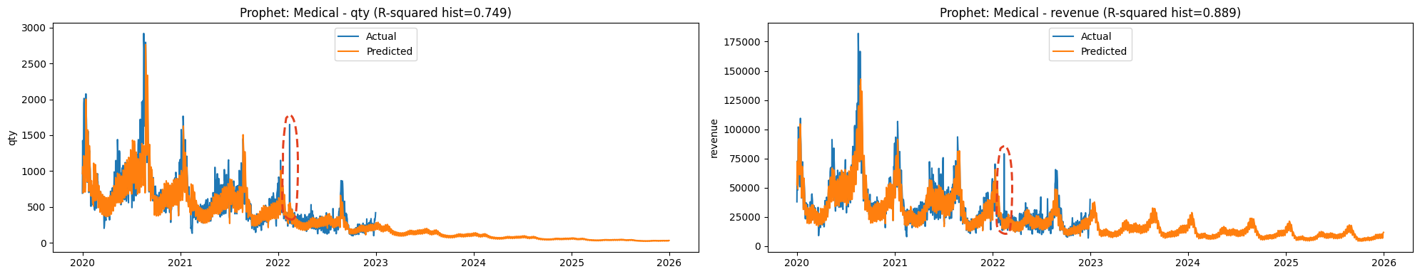
Weekly patterns in Science & Technology are more consistently detectable by the model in the holdout dataset, while Medical qty appears less stable, with a single atypical spike in January 2022 where the increase in units is harsher than the increase in revenue (see the graphs below). One possible explanation is a temporary change in average selling price (e.g., discounting or a promotion), but this has not been verified. Before any promotion-related feature is added to the model, the spike should be investigated by checking the implied unit price (revenue/qty) and, if available, reviewing order-level details for that period.
Below are the full charts forecasted through 2026 (3 years) on a weekly basis. However, it is not recommended to rely on forecasts beyond about one year. These models were trained on only three years of data, which limits how well they can learn stable year-to-year patterns and rare disruptions. As the horizon extends, uncertainty grows and the predictions become less dependable (i.e., the model can drift if the underlying demand pattern changes).
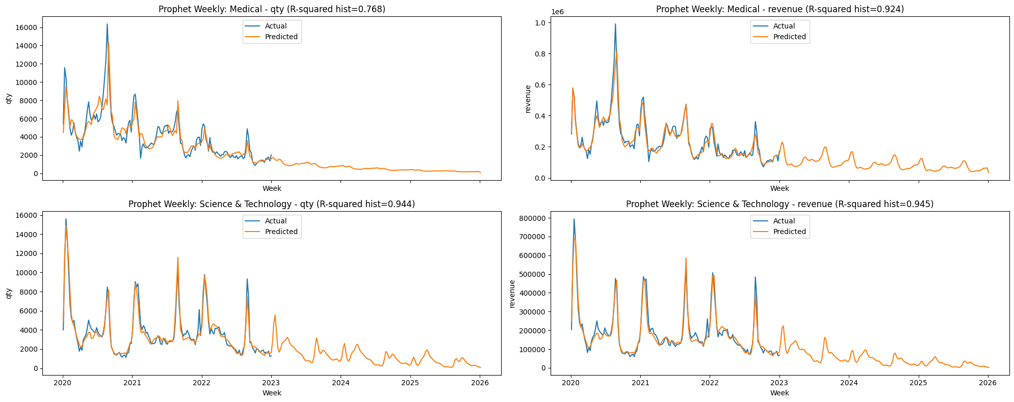
In particular, Medical qty should be treated with extra caution. Compared with the other series, it shows weaker fit and more irregular spikes, so the model is less confident about its baseline level and peak timing. As a result, the long-range projection for Medical qty may drift more as the forecast horizon increases.
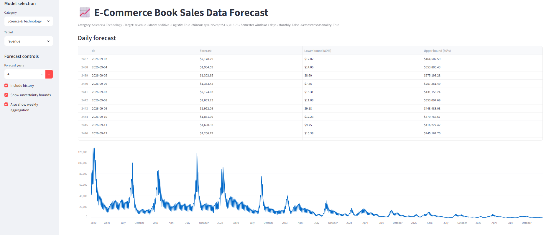
Deployment: Streamlit App
This project includes a lightweight Streamlit app for interactive forecasting. The app loads the pre-trained Prophet models (as joblib) saved in the models/ folder (one model per category x target) and generates daily forecasts (plus optional weekly aggregation). Because the models were trained on log1p(y), the app automatically applies expm1() to convert predictions back to the original scale. For targets trained with logistic growth, the app also applies the saved floor/cap values during prediction to ensure consistent behavior with training.
Folder / file requirements
Before running the app, confirm these files exist:
app.py— the Streamlit application entrypointmodels/— contains model artifacts saved as joblib:model__<category>__<target>.joblib
requirements.txt— includes Streamlit + Prophet dependencies
Example model files:
models/model__medical__qty.joblibmodels/model__medical__revenue.joblibmodels/model__science_and_technology__qty.joblibmodels/model__science_and_technology__revenue.joblib
How to run locally
Using the same virtual environment, start this streamlit app:
streamlit run app.py
Recommendations
Here are some recommendations to improve the performance of the models:
- Add more detailed calendar features (major/minor holidays, academic breaks, exam weeks). Right now, holidays are treated as one general effect, and semester patterns are inferred from demand spikes. This works as a starting point, but not all calendar events have the same impact. A better approach is to label holidays and academic periods more specifically, like separating major holidays, minor breaks, finals week, or orientation week. This helps the model learn how each one affects demand differently, instead of averaging them all together.
- Add non-seasonal drivers (price/promotions, new editions, curriculum changes) and validate them first.
Some spikes may be caused by discounts, product-mix shifts, or operational constraints. A simple first check is implied unit price (
revenue/qty). If unit price drops while quantity jumps, the period may reflect a promotion. Where possible, confirm this using order-level fields (discount codes, campaign tags, basket size) or operational records (inventory notes, release dates).- When direct drivers are missing, use change-point methods (e.g., CUSUM) to flag sudden shifts in demand that may indicate price changes, supply constraints, or new editions. However, treat these only as investigation leads, and then verify them with real world records before adding them as drivers.
- When drivers are available, model them as continuous regressors (discount rate, ad spend, traffic, share of discounted orders), since effects are rarely binary. Prophet can include regressors, but if impacts are nonlinear or interact with seasonality, models like LightGBM or XGBoost may perform better.
- Tune hyperparameters more efficiently (random search or staged tuning). Expanding the grid may be an option as well, but it can become computationally expensive very quickly. Random search tends to identify strong parameter combinations more quickly. Staged tuning is another practical approach, where, for example, one can start with tuning trend flexibility, then seasonality priors, and finally adjust optional seasonalities and event-related parameters. Alternatively, use Bayesian optimizers like Optuna for hyperparameter tuning.
- Use time-series cross-validation for a more reliable evaluation. A single time-based holdout is simple and easy to explain, but results can depend heavily on the chosen cutoff. Rolling / walk-forward cross-validation (multiple cutoffs, fixed forecast horizon) gives a more stable view of how the model performs across different periods. However, there’s a higher compute cost to CV (i.e., slower computation), since CV multiplies training runs and can become expensive when combined with large grids.
- Model peaks more directly.
Applying
log1ptransformation improves numerical stability, but can flatten sharp peaks once reversed. For operationally critical peak periods (e.g., semester starts), the model should rely more on clearly defined events rather than general seasonal terms. Using verified academic calendars and defining distinct event types (such as “semester start” and “semester break”) can help capture these demand surges more accurately. In some cases, event windows should be adjusted by category to reflect specific patterns. - Re-evaluate additive vs. multiplicative seasonality as more history becomes available. With only 3 years of data, it is difficult to learn stable year-to-year behavior, so the model may select a seasonality mode that fits the holdout period but does not generalize long term. For example, Medical may look multiplicative in this window because the overall level shifts, but with more years of history it could behave more like an additive series. As data accumulates, this should be re-tested using rolling backtests across multiple cutoffs and by checking whether the preferred seasonality mode remains consistent across years.
- Use weekly forecasting once more history is available. Weekly aggregation reduces day-to-day variability and generally yields smoother, more stable long-range forecasts. This is particularly useful when daily demand is volatile or hard to predict. In the current dataset (2020-2022), daily modeling was preferred due to limited history, but weekly modeling becomes more feasible and effective as the time range expands.